Shapley and Owen values for model output explainability: a hands-on case study

Originating from cooperative game theory, these values offer a robust framework for analyzing the predictions made by models. They allow us to identify the specific contributions of each feature involved in a certain prediction, highlighting how much each feature influences the outcomes. Additionally, they reveal the complex interactions between features, providing a deeper understanding of their combined effects.

By utilizing these values, we can achieve clearer insights into the mechanisms of machine learning models, ultimately fostering greater trust and understanding of their applications.

This article presents a case study using SHAP’s PartitionExplainer method. With this exercise, we are going to compute Owen values for a two-level stacking ensemble model on a public dataset containing strongly correlated features. By incorporating feature coalitions, we find that the differences between Shapley and Owen values can significantly impact model interpretation and computational efficiency, as grouping features reduces the number of combinations needed for calculation.

Hands-on: Dataset description

This article’s “Hands-on” sections provide step-by-step explanations of the exercise, including Python code snippets. Here, we begin by importing the required libraries.

import shap
import numpy as np
import pandas as pd
import seaborn as sns
import scipy.cluster.hierarchy as sch
from scipy.spatial import cKDTree
from scipy.spatial.distance import squareform
from sklearn.model_selection import train_test_split
from sklearn.metrics import mean_squared_error
from sklearn.pipeline import make_pipeline
from sklearn.linear_model import LinearRegression
from sklearn.tree import DecisionTreeRegressor
from sklearn.ensemble import StackingRegressor

For this case study, we use the California Housing public dataset to predict the median house value for California districts, expressed in hundreds of thousands of dollars. This regression dataset contains 20,640 records and 8 columns.

X, y_ = shap.datasets.california()

Before entering the modeling stage, we created a new variable called “spatial_density” using the “Latitude” and “Longitude” features to capture the geographic distribution.

spatial = cKDTree(X[["Latitude", "Longitude"]])
X["spatial_density"] = spatial.query_ball_point(X[["Latitude", "Longitude"]], 0.005, return_length = True)

Afterward, we removed “Latitude” and “Longitude” to prevent potential bias. Additionally, the target variable (median house value) was transformed using a logarithmic function to stabilize variance and improve model performance.

y = pd.DataFrame(np.log(y_), columns=["target"])

xtrain, xtest, ytrain, ytest = train_test_split(
    X.drop(columns=["Latitude","Longitude"]), y,
    test_size=0.1, random_state=42
)

Given the relationships among certain features, we anticipate forming feature coalitions. For example, “AveBedrms” and “AveRooms” are strongly correlated, as both are associated with the average size of houses in the area, while “MedInc” and “Population” are more independent since areas with high populations do not necessarily have higher or lower median incomes.

## Features correlation

sns.clustermap(
    round(xtrain.corr(),2), method="complete", cmap="RdBu",
    annot=True, annot_kws={"size":9}, vmin=-1, vmax=1, figsize=(8,8)
)

Correlation analysis shows that most feature correlations (in absolute value) range from near zero to 0.85, indicating inter-feature correlations.

Hands-on: Model architecture

In this hands-on, we use a two-level stacking ensemble model with two decision trees as base learners and a linear regression as the meta-learner.

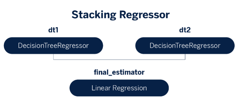
## Model architecture

params_base_learner_1 = {
    "max_depth": 3,
    "random_state": 42
}

params_base_learner_2 = {
    "max_depth": 7,
    "random_state": 42
}

base_learner_1 = DecisionTreeRegressor(**params_base_learner_1)
base_learner_2 = DecisionTreeRegressor(**params_base_learner_2)
meta_learner = LinearRegression()

base_estimators = [("dt1", base_learner_1), ("dt2", base_learner_2)]

model = StackingRegressor(
    estimators=base_estimators,
    final_estimator=meta_learner,
    cv=5,
    n_jobs=-1,
    verbose=5,
)

model.fit(xtrain, np.ravel(ytrain))

Model performance evaluated with the mean squared error (where lower values indicate better performance) shows a slight improvement in the stacking ensemble (0.1249) over the individual base learners, with decision trees scoring 0.1626 and 0.1259.

Shapley Values: Understanding individual contributions

Shapley values are a method from cooperative game theory that allows us to measure each feature’s individual contribution to a model’s prediction.¹ Think of the model’s prediction as a “reward” that needs to be fairly distributed among “players” (the features). By calculating Shapley values, we determine how much each feature contributed to the prediction by seeing how the prediction changes when we add or remove that feature from various subsets of features.

To calculate Shapley values, we use a value function representing the model’s prediction based on any subset of features. This function lets us measure how much the prediction changes when a particular feature is added to a subset, capturing the marginal contribution of each feature².

Because the model’s prediction depends on all features—even those not in the subset we’re focusing on—we use marginalization to account for the remaining features by averaging their possible values. This lets us isolate the specific impact of the features in our subset.

The Shapley value for a feature is computed by averaging its marginal contributions across all possible subsets of features. This ensures that each feature’s contribution is fairly represented. However, calculating Shapley values for all subsets becomes computationally intense as the number of features increases since there are exponentially many subsets to consider.

To simplify this, we use Monte Carlo sampling to approximate Shapley values by randomly sampling subsets of features rather than evaluating them all. This method involves comparing the model’s predictions on random subsets with and without a specific feature and then averaging these differences across samples of records to estimate the feature’s contribution.

Hoeffding’s inequality: Ensuring accuracy in sampling

When estimating Shapley values through sampling, it’s important to evaluate how close these approximations are to the true values. Hoeffding’s inequality helps us by providing a statistical guarantee: it bounds the probability that the sampled-based Shapley values will deviate from the true Shapley values by more than a specified amount.

By applying Hoeffding’s inequality, we can establish that, for a sufficiently large number of samples K, the probability that our Shapley value estimate deviates from the actual value by more than a small error margin ∈ becomes very small. This is given by:

This inequality shows that as we increase K, the probability of significant error decreases, making our Shapley value estimate more reliable. Therefore, Hoeffding’s inequality guides us in choosing a suitable sample size to achieve an acceptable accuracy level in Shapley value estimation.

Hands-on: Shapley values for the California Housing dataset

In our hands-on experiment with the California Housing public dataset, we use SHAP’s KernelExplainer, which supports stacking ensemble models. KernelExplainer estimates Shapley values by sampling subsets and comparing predictions with and without each feature, applying the above principles. Although KernelExplainer is flexible, it assumes feature independence, which can lead to slight biases when features are correlated.

## Shapley values through KernelExplainer

K = 2520   # From Hoeffding with p=7, a=-2, b=2, alpha=0.01, epsilon=0.1 

background_data = shap.sample(xtrain, K, random_state=0)
fn = lambda x: model.predict(pd.DataFrame(x, columns=list(xtrain.columns)))

ker_expl = shap.KernelExplainer(fn, background_data, link='identity')
shap_vals_ker = ker_expl(xtest.sample(500, random_state=37))

shap.plots.bar(shap_vals_ker)

A key limitation of KernelExplainer is that it ignores dependencies between features, even when they are correlated. This is because it uses marginal sampling rather than conditional sampling. Consequently, the Shapley values calculated with KernelExplainer may be biased by its assumption that features are independent. Given our experiment’s natural grouping of features, Owen values may have been a more suitable choice from the start, as they can account for feature interactions.

Owen Values: Accounting for feature interactions

Like Shapley values, Owen values aim to fairly distribute the model’s prediction among features.³ However, instead of evaluating features individually, Owen values allow us to create coalitions of features that act together.⁴ For example, features “AveBedrms” and “AveRooms” are strongly correlated, so evaluating them as a coalition rather than separately makes sense.

To calculate Owen values:

1. We first form coalitions based on related features.
2. Then, we treat each coalition as a single “player” in the cooperative game, calculating the Shapley value for each coalition.
3. Finally, within each coalition, we distribute the coalition’s Shapley value among individual features based on their individual contributions within the coalition.

This two-step process (calculating Shapley values for coalitions, then distributing within each coalition) ensures that Owen values accurately reflect both individual and collective contributions, especially when features are interdependent.

Hands-on: Owen values for the California Housing dataset

Continuing with our hands-on, to compute Owen values in practice, we can use SHAP’s PartitionExplainer, which allows us to specify feature coalitions based on their interactions. By clustering correlated features into groups, we can create coalitions that better reflect real-world dependencies, capturing their collective influence.

## Correlation-based clusters of features
dist = 1 - np.abs(xtrain.corr())   # distance matrix
condensed = squareform(dist)
clust = sch.linkage(condensed, method="complete")

# Equivalently, we can use the following one-line code
# clust = shap.utils.hclust(xtrain, metric="correlation")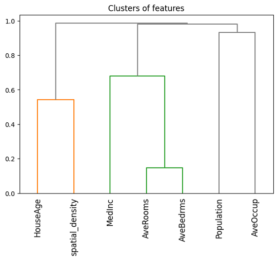

Next, we specify these feature groups for the PartitionExplainer through the clustering parameter, as shown below.

## Shapley values through PartitionExplainer

masker = shap.maskers.Partition(xtrain, clustering=clust)

part_expl = shap.PartitionExplainer(fn, masker)
shap_vals_part = part_expl(xtest.sample(500, random_state=37))

shap.plots.bar(shap_vals_part, clustering_cutoff=0.75)

Conclusions

In machine learning explainability, choosing between Shapley and Owen values is a strategic decision. Shapley values excel in analyzing independent contributions, while Owen values are better suited for capturing interactions within feature groups. This distinction is crucial when dependencies exist, as Owen values provide a more accurate reflection of joint influences.

When features are correlated, the use of KernelExplainer from the SHAP library can lead to biased results, since this method assumes all features are independent. In cases where features naturally form groups, Owen values offer a better alternative by accurately capturing feature interactions through grouped coalitions.

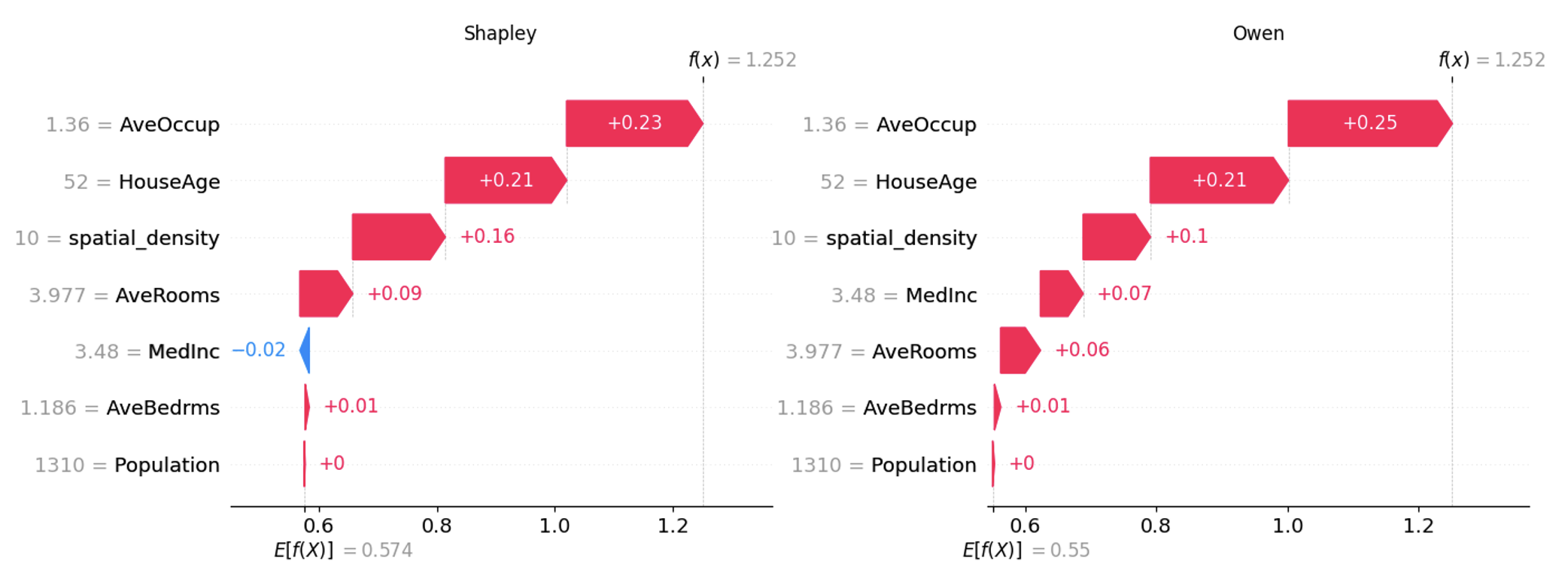
Combining Shapley and Owen values is beneficial in complex models with independent and interdependent features. This hybrid strategy enhances model transparency and trust while empowering data scientists to deliver explanations that align with the data structure, enabling more informed and reliable decision-making.

References

- Scott, M., & Su-In, L. (2017). A unified approach to interpreting model predictions. Advances in neural information processing systems, 30, 4765-4774.↩︎
- Molnar, C. (2023). Interpreting machine learning models with SHAP.↩︎
- Owen, G. (1977). Values of games with a priori unions. In Mathematical economics and game theory: Essays in honor of Oskar Morgenstern (pp. 76-88). Springer Berlin Heidelberg. ↩︎
- Giménez Pradales, J. M., & Puente del Campo, M. A. (2019). The Owen and the Owen-Banzhaf values applied to the study of the Madrid Assembly and the Andalusian Parliament in legislature 2015-2019. In Proceedings of the 8th International Conference on Operations Research and Enterprise Systems-Volume 1: ICORES, 45-52, 2019, Prague, Czech Republic (pp. 45-52). Scitepress. ↩︎