BBVA AI Factory | Graph-based feature engineering: a hands-on exercise with mercury-graph

Mercury-graph is one of the repositories of our open-source library, Mercury. In this hands-on, we will model data as a graph and engineer features to enhance model performance

Graphs have emerged as a fundamental tool for understanding complex systems across various domains. By representing entities as nodes and relationships as edges, graphs offer a versatile framework for characterizing, analyzing, and visualizing interactions between objects of interest. This approach facilitates the identification of patterns, trends, and anomalies within intricate datasets.

The adoption of graph-based analysis has been increasingly prominent at BBVA. This article introduces BBVA’s open-source implementation for automatically generating graph-based features to enhance model performance.

To make the methodologies discussed in this article more accessible and practical, we have made our code publicly available on mercury-graph. This resource enables readers to run their own experiments and apply these concepts to their specific case studies, thereby promoting a deeper understanding and ensuring the reproducibility of our findings.

Context of the problem

Machine learning models’ effectiveness depends on relevant patterns within the underlying data. Certain patterns, however, particularly those derived from relationships within a network, can be challenging for models to learn without explicitly modeling the data as a graph. Incorporating graph-based variables into the feature set enables models to uncover complex patterns that might otherwise be overlooked, thereby improving their overall performance.

This idea is summarized by the famous quote from linguist John R. Firth: “You shall know a word by the company it keeps”. Just like a word’s meaning can be inferred from the words around it, we can learn a lot about a person by looking at who they’re connected to. In a network, the people (or nodes) with whom someone interacts often reflect shared interests, habits, or backgrounds. That’s the intuition behind aggregating information from neighbors in a graph — it helps the model pick up on patterns that aren’t obvious from an individual’s features alone.

Suppose we’re training a supervised model. Prior to the introduction of graph-based variables, our model was unable to see any further than each observation’s own attributes. In contrast, once we model the data as a graph, we enable our model to use the information surrounding each observation.

In a traditional dataset, each observation has its own set of attributes (income, expenses, and so on). In order to engineer graph-based features, we must model the data as a graph, use its network structure to aggregate each node’s information and pass it on to a nearby neighbor. This way, your neighbor receives your information whilst you receive that of your neighbors.

This process is formally known as message passing because we pass our neighbors’ messages (features) using the graph’s edges. Multiple frameworks can do this, with PyTorch Geometric being the most popular implementation. Unfortunately, such implementations were developed to run on a single computer, and real-world graphs are usually too large to fit in a single memory. We therefore developed our own distributed solution and published it in mercury-graph ¹.

Hands-on: Graph features with mercury-graph

We start with a standard dataset where each observation has a set of attributes and a target. Our goal is to boost the model’s performance by adding features containing information about a node’s neighbors. The principle that underlies this idea is that our behavior is influenced by those around us.

In order to add features of the people in our surroundings, we first need to determine who’s connected to whom. In graph terms, this means defining a set of edges that model pairwise relationships between nodes. We will use the edges to find everyone’s neighbors, fetch their features, apply some aggregation function (like an average), and pass this information back to the original node.

In addition to the node-level attributes in the original dataset, these graph-based features provide richer context, allowing the model to uncover hidden patterns in the data and ultimately improve its predictive performance.

To put things into perspective, we’ll use the BankSim dataset, an open-source dataset representing transactions between customers and merchants. Each node is either a customer or a merchant, and the two are connected by a transaction amount. Only customers have attributes like gender and age (merchants do not have attributes).

Hands-on: Setting up the environment

Let’s start off by importing the necessary dependencies and setting up a PySpark session.

# Imports
import pandas as pd
import mercury.graph as mg
from pyspark.context import SparkContext
from pyspark.sql import SparkSession


# Set up PySpark session
spark = (
    SparkSession.builder.appName("graphs")
   .config(
        "spark.jars.packages",
        "graphframes:graphframes:0.8.3-spark3.5-s_2.12"
    )
   .getOrCreate()
)

We now proceed to load and clean the data.

# Declare paths
PATH = (
   "https://raw.githubusercontent.com/atavci/fraud-detection-on-banksim-data/refs/"
   "heads/master/Data/synthetic-data-from-a-financial-payment-system/"
   "bs140513_032310.csv"
)

# Read data
df = pd.read_csv(PATH, quotechar="'")


# Declare total amount transacted per customer
df["total"] = df.groupby("customer")["amount"].transform("sum")


# Drop observations where age or gender are unknown
df = df[df["age"].ne("U") & df["gender"].isin(["M", "F"])]


# Cast age and gender to integer types
df = df.assign(
   age=df["age"].astype(int),
   female=df["gender"].eq("F").astype(int)
)

In its original form, the data shows connections between customers and merchants, but only customers have attributes. To make the data more useful, we need to link customers to each other using merchants as middlemen. This is important because our goal is to pass messages between connected nodes, and that wouldn’t work if we left the data as it is (because merchants don’t have attributes!).

# Init edges as a subset of df
edges = (
   df[["customer", "merchant"]]    # Select columns
   .drop_duplicates(keep="first")  # Ignore multigraph structure
   .reset_index(drop=True)
   .sample(5000, random_state=42)  # Downsize for this example
)

# Self join on merchant to get customer-customer relations
edges = edges.merge(right=edges, how="inner", on="merchant").drop(columns="merchant")
edges.columns = ["src", "dst"]  # Rename columns
edges = edges[edges["src"] != edges["dst"]]  
# Drop self-loops

Our next step is to declare a mercury-graph object using the tables we just loaded.

# Declare graph using vertices and edges
g = mg.core.Graph(
   data=edges,
   nodes=vertices,
   keys={"directed": False}
)

We now have a mercury-graph object that represents the network. Our goal is to generate new features by taking the information from its vertices and passing them to other nodes through the structure defined by its edges.

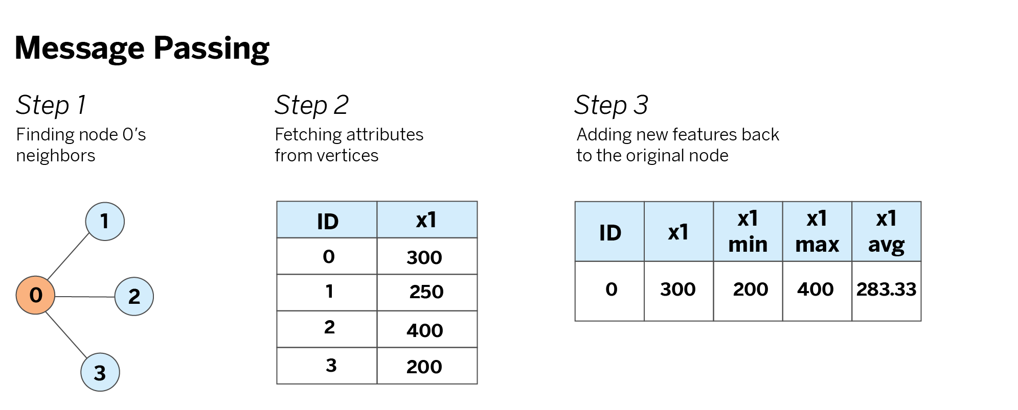
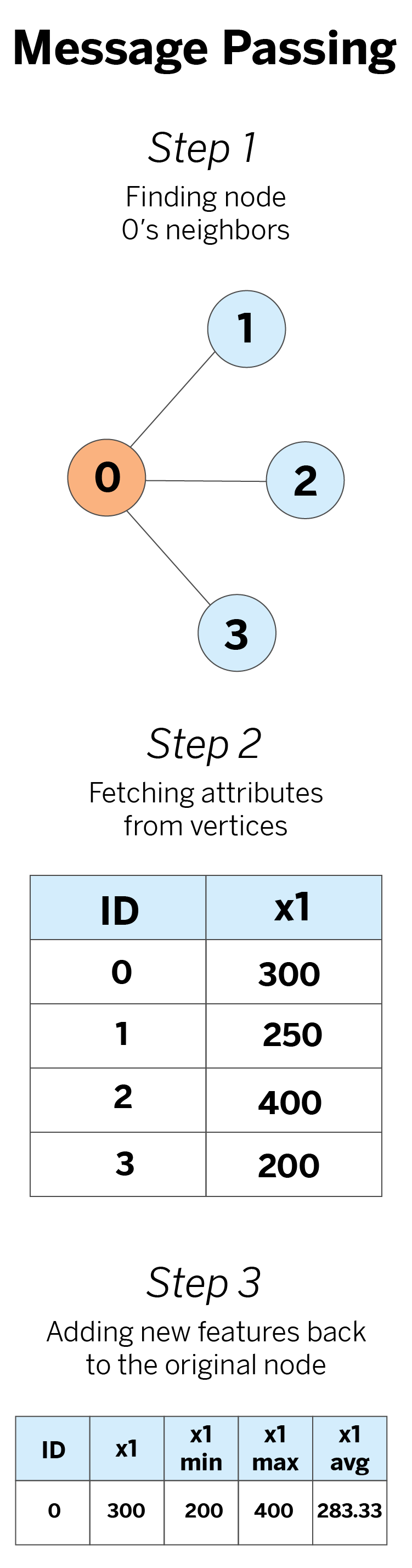
Message passing for a single node

First, we use the graph’s edges to find the neighbors of the node of interest. For example, if we’re interested in generating new features for node 0, we use the edges to find its neighbors 1, 2, and 3. Then, we look up the neighbors in the graph’s vertices and fetch their individual attributes.

Finally, we aggregate the attributes we fetched with our desired aggregation functions (minimum, maximum, and average in this example) and add this new information to the original node.

Hands-on: Message passing with mercury-graph

We developed GraphFeatures, a class that implements a distributed version of this process. It receives a Mercury Graph object and engineers graph-based features for all the nodes in the network.

# Init GraphFeatures instance
gf = mg.ml.graph_features.GraphFeatures(
   attributes=["age", "female", "total"],  # Features to be aggregated
   agg_funcs=["min", "avg", "max"]  # Aggregation functions to be applied
)

# Fit instance
gf.fit(g)

In the code snippet above, attributes represents the node-level attributes we want to aggregate, and agg_funcs represents the aggregation functions we want to apply to said attributes. Upon fitting the instance, the class produces a cartesian product of both arguments so that each attribute is passed to all the aggregation functions. In other words, each attribute will be passed to each function and the following features will be engineered:

age_min: Minimum age of first-order neighbors
age_avg: Average age of first-order neighbors
age_max: Maximum age of first-order neighbors
female_min: Minimum value for female among first-order neighbors (a value of zero implies that the node has at least one male neighbor)
female_avg: Average value for female among first-order neighbors (interpreted as the share of neighbors who are female)
female_max: Maximum value for female among first-order neighbors (a value of zero implies that the node has no female neighbors)
total_min: Minimum amount transacted of first-order neighbors
total_avg: Average amount transacted of first-order neighbors
total_max: Maximum amount transacted of first-order neighbors

It is important to note that in this dataset, information regarding gender is binary, (1 for female and 0 for male). Consequently, explicitly including both female and its complement (male = 1 − female) would lead to perfect collinearity. Thus, we only incorporate female in our model to avoid redundancy and multicollinearity issues.

We can now access the newly added node_features_ property to retrieve the engineered features.

# View generated attributes
gf.node_features_.show(5)

The purpose of these new features is to incorporate them into the feature set to enhance the model’s performance. Prior to their introduction, the model can only learn from node-level attributes. By incorporating these features, the model can also learn from hidden patterns that can only be inferred from the graph’s structure.

Moving to higher orders

As a technical note, a node does not need to be directly connected to another node in the graph for them to be considered neighbors. To see this, think of your neighbor’s neighbor; are they not your neighbors too? Two nodes connected through an intermediary are known as second-order neighbors because they are connected through a two-step path. Likewise, third-order connections represent nodes connected through three-step paths and so on.

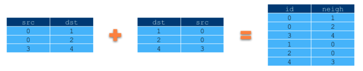
The first step is using the graph’s edges to determine the neighbor relationships – not for a single node, but for all nodes at once. In an undirected graph, we achieve this by taking the edges table and concatenating a copy of itself with the source and destination columns swapped (src becomes dst and dst becomes src). The result is what we call the first-order neighbors table, which serves a similar purpose to an adjacency matrix but is stored more efficiently because of its longitudinal form.

Figure 2. Creating the first-order neighbors table by concatenating `edges` with itself

Fetching your second-order neighbors is a simple task. All we need to do is join the first-order neighbors table with itself using neigh as the join key. Similarly, we can join the neighbors table with itself one additional time to get the third-order neighbors table.

Technically, we can do this to find all n-order connections, but this process becomes computationally expensive because it involves joining the edges table (which is presumably very large) with itself n consecutive times. Additionally, it’s hard to argue that third-degree (or greater) connections truly affect your behavior because of the distance between yourself and your neighbors’ neighbors’ neighbors.

Regardless, our implementation is capable of generating features of any order. As previously mentioned, we calculate the n-th-order neighbors table by recursively joining the first-order neighbors table with itself. This table is the concatenation of edges with itself (a very large table on its own); hence, spark’s logical plan will overflow your memory.

The secret to preventing the logical plan from exploding is to checkpoint the first-order neighbors table as well as the current iteration’s result of the self-join. This prevents our memory from overflowing and allows us to aggregate messages of any order.

Conclusions

The effectiveness of machine learning models depends heavily on their ability to capture relevant patterns within the data. Incorporating graph-based variables into our feature space enables our model to leverage complex customer relationships, enhancing its predictive power. Prior to the inclusion of these graph-based variables, our models are limited to evaluating each observation in isolation.

However, by modeling the data as a graph, we allow the model to incorporate insights from the network’s structure, significantly improving its performance. This demonstrates the value of graph-based feature engineering in revealing hidden patterns and improving model performance.

Graph-based feature engineering: a hands-on exercise with mercury-graph