Bridging the gap: Demystifying black-box algorithms with Mercury-explainability
Explainability seeks to reduce the distance between users and algorithmic complexity by providing the necessary tools to understand the decisions made by AI systems.
In this context, it is essential to establish a framework that allows us to create traceable, auditable, and interpretable algorithms so that the consumers of these systems can understand how they operate. In addition, there is a clear need to employ methods and techniques that allow data scientists to observe algorithmic behavior to refine machine learning models.
XAI for understanding algorithmic decisions
The concept of eXplainable Artificial Intelligence (XAI) was born to understand the logic behind the decisions suggested by algorithms. It aims to reduce the uncertainty inherent in the operation of machine learning models, especially deep learning models, and thus improve our understanding of what processes have been followed to arrive at a specific result. We could say that they help to convert opaque systems (black boxes) into clear and justifiable structures that allow us to understand their decisions better.
Explainability has different scopes and benefits in terms of how it serves people. On the one hand, it helps those without a technical background understand how algorithms work, positively affecting their confidence in using these technologies. This is especially useful within business teams: it strengthens their relationship with advanced analytics and helps them gain confidence in their capabilities. In this approach, business units can corroborate whether a model suits a particular use case, allowing them to discern.
On the other hand, it helps data scientists and engineers explain how algorithms behave at different levels for sets of predictions and/or individual predictions. This can lead to the detection of possible errors in the performance of the models, thus allowing them to refine them, improve their performance, and create more robust algorithms.
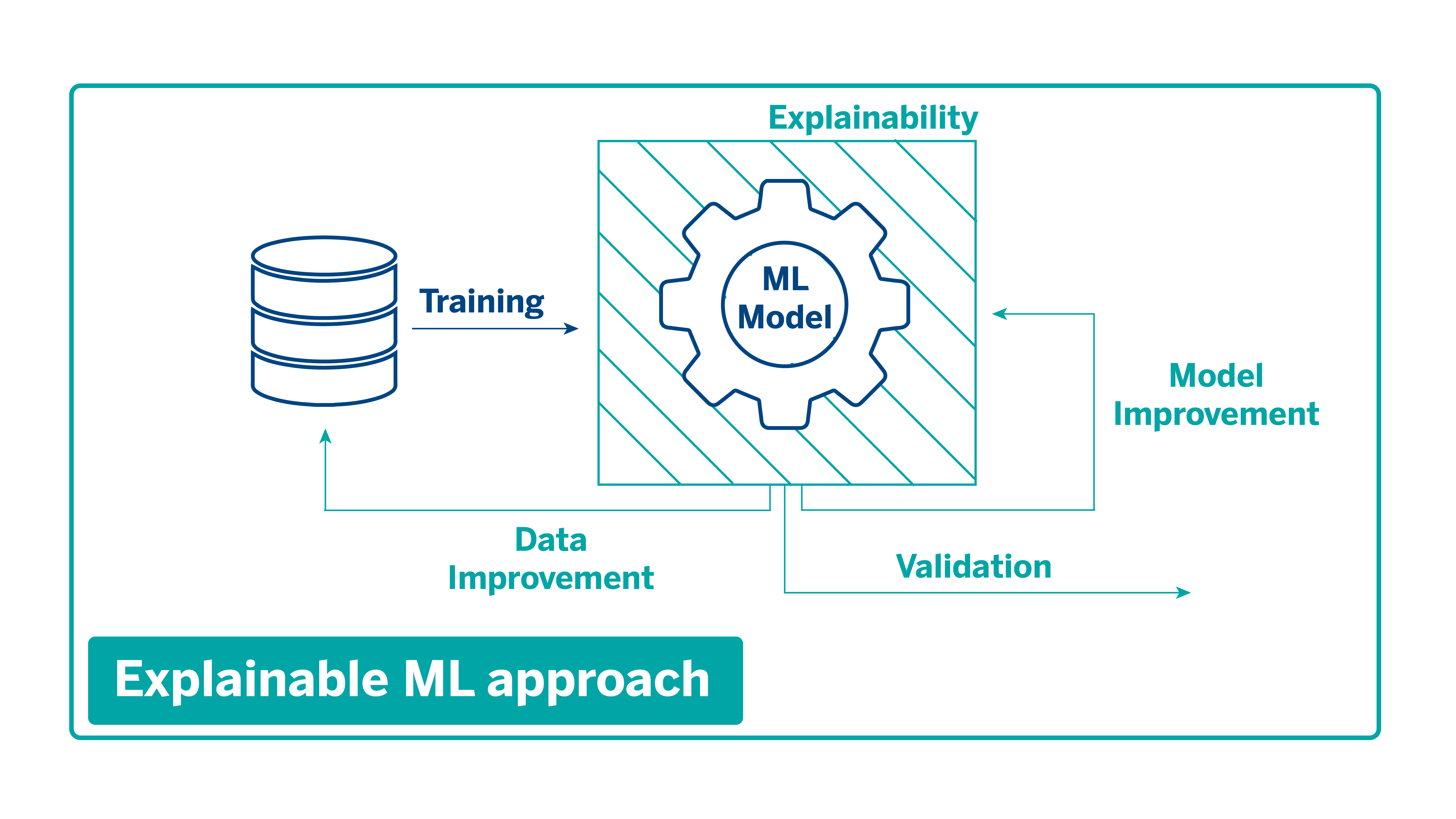
Explainability techniques help debug models in the evaluation phase, identifying problems in the data and the models themselves so that they can be improved and retrained until they can be validated as reliable and deployed in production environments.
Explainability as a working methodology in BBVA AI Factory
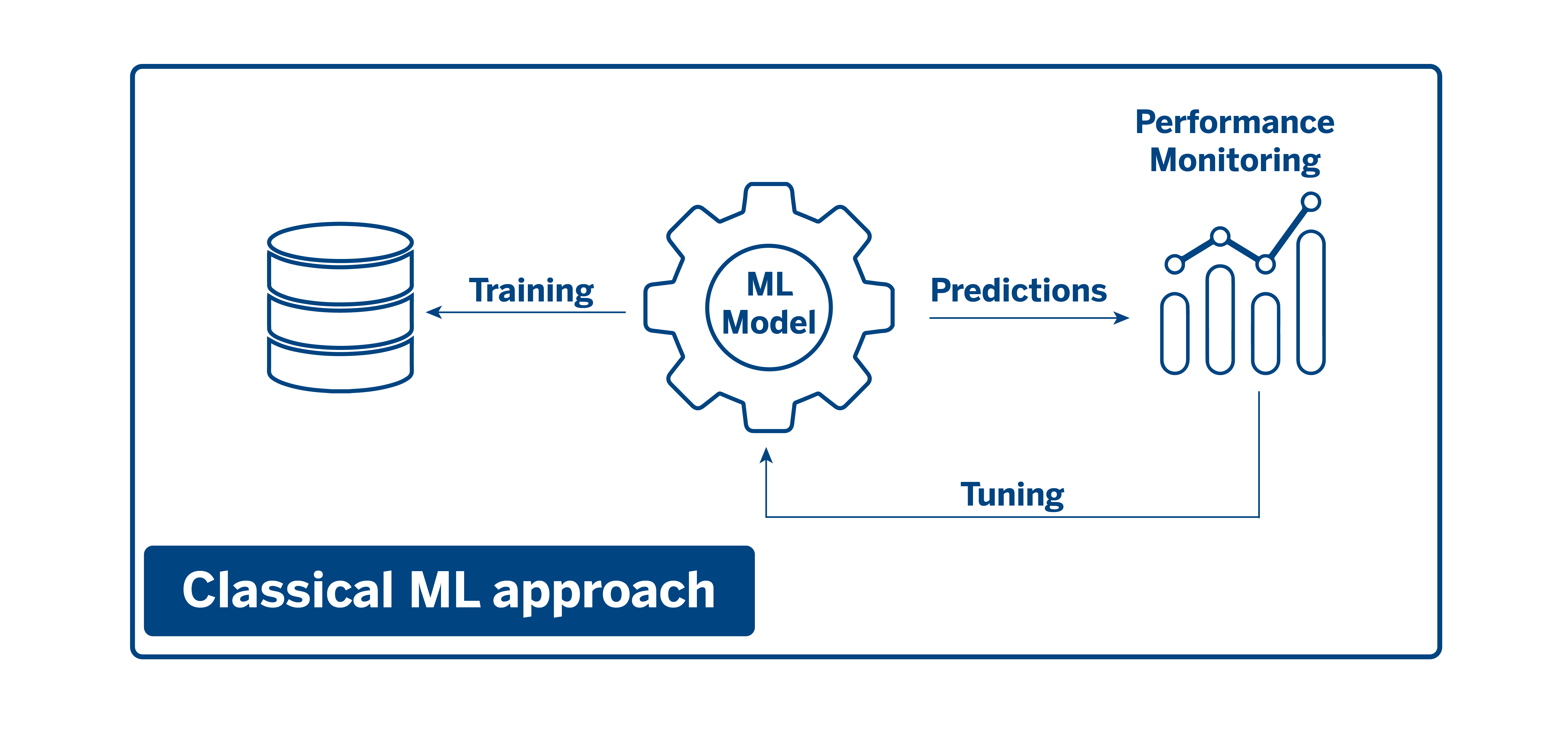
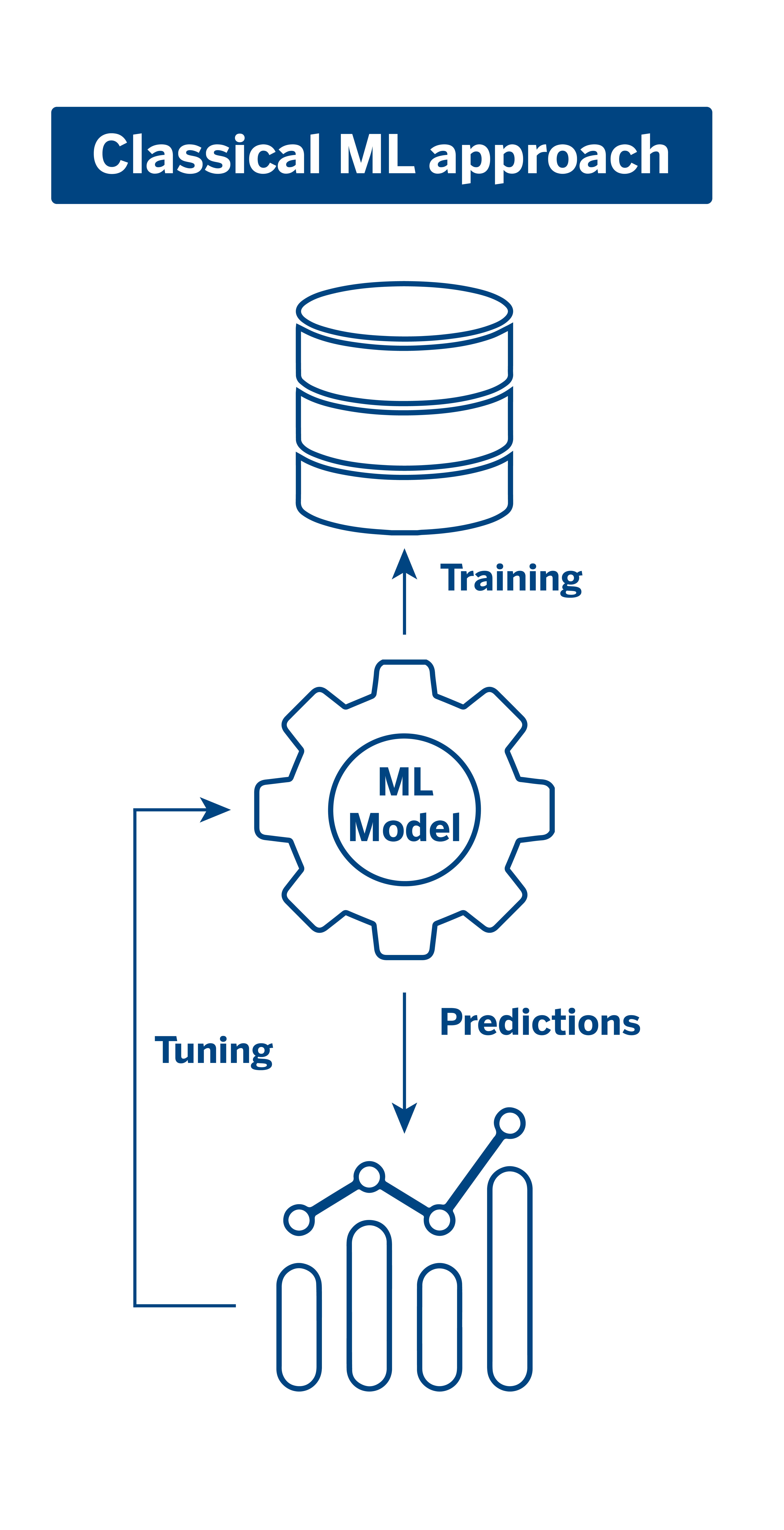
Explainability comprises a series of techniques and tools that we use in AI Factory and have become part of our work methodology. From a classical perspective, models were trained with data, these models made predictions, and then their performance was monitored and then refined and retrained.


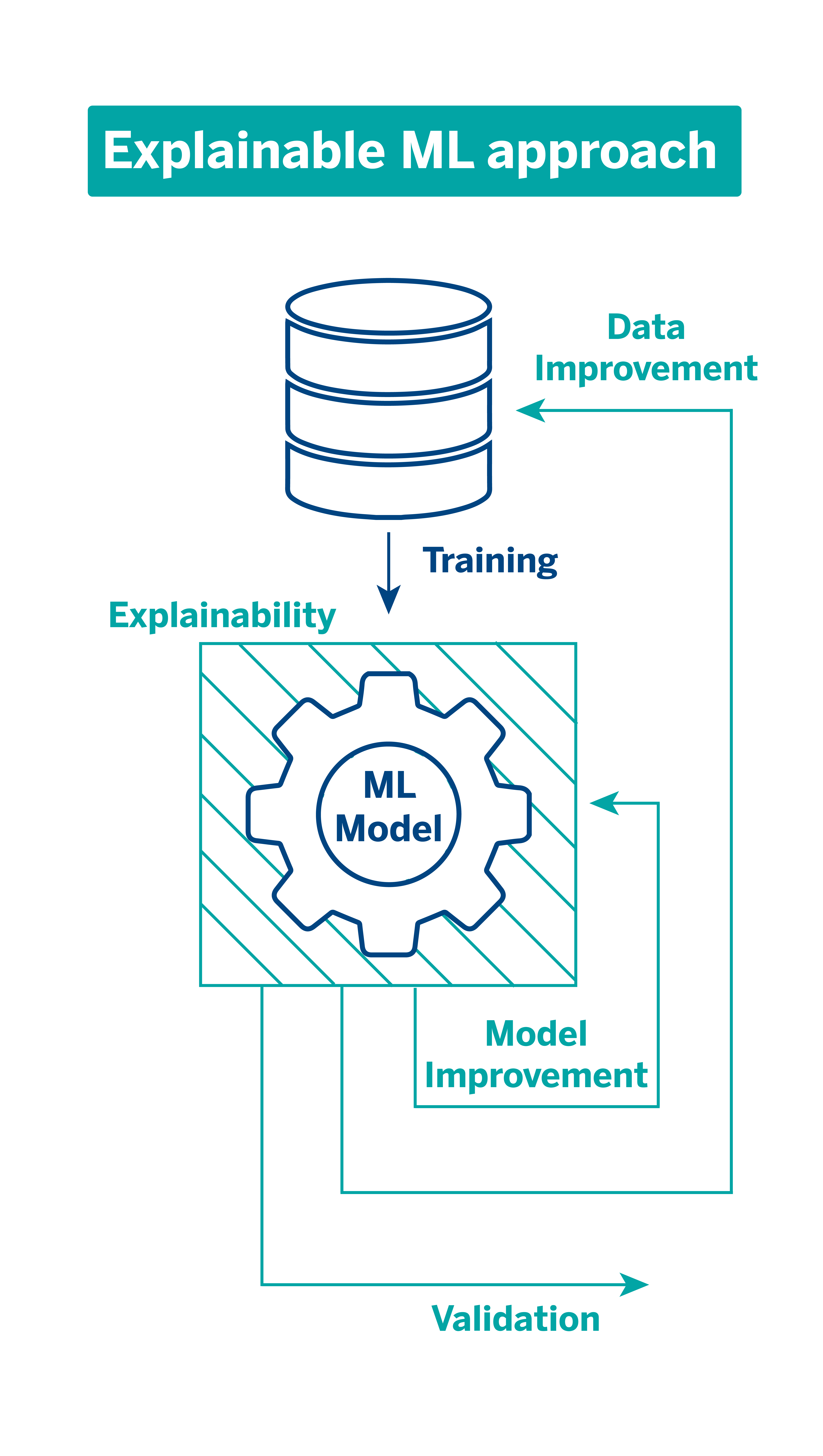
With the emergence of explainability and interpretability techniques, an explainability module comes into play during the training process, from which iterations are performed on both the data and the models. This module considers factors such as the analysis of the predictions or the importance of the different variables in the model, among other elements that help us identify biases or possible errors before deploying them in production.


This module, called mercury-explainability, is available in open-source for anyone who wants to integrate explainability techniques into their models.
Mercury-explainability: Explainability module available to everyone
As mentioned in a previous article, BBVA AI Factory developed the Mercury code library to facilitate the reuse of analytical components within BBVA. Recently, part of this library has been released as open source for the whole community. One of the released packages,mercury-explainability, contains components that facilitate the explainability of artificial intelligence models.
Mercury-explainability contains methods not implemented in other widely adopted open-source explainability libraries such as SHAP or LIME. These components are prepared to work with models viewed as “black boxes”; that is, they can be applied to different types of models. In addition, some of these components can be used for pyspark models.
Global and local algorithms available in mercury-explainability
In the library, we can find both global and local explainability methods. Global explainability methods provide us with information on how the model works in a general way, the whole picture. These methods indicate, for example, which model inputs are usually the most important or how changes in the values of a model input impact the predictions in a general way.
On the other hand, local explainability methods try to explain a model’s decision for a particular instance indicating, for example, which inputs in the model have had the most significant impact on its prediction.
Global explainability methods |
|
| Partial Dependence Plots (PDP) | This method shows plots demonstrating the average effect of changing one of the inputs on the model prediction. Thus, we can confirm how the prediction varies depending on the input data. For example, suppose we have a model that predicts the probability of default when granting a loan. In that case, it can help us to understand that our model tends to decrease the probability of default when the model input “monthly income” increases. |
| Accumulated Local Effects (ALE) Plots | This method is very similar to PDPs in that they show how model inputs affect the prediction on average. ALE Plots tend to be more reliable in cases with correlations between different model inputs. |
| Shuffle Feature Importance | This method is model-independent, so we can use any type of model to adopt it. It consists of estimating the importance of the different inputs of a model in a general way. The importance of a model input is measured by performing a “shuffle” (random order) of the values of this input and measuring how it impacts the model error. If it is an important input, the model error will increase because of the shuffle. However, if the model error remains the same, this input is unimportant to the model. |
| Clustering Tree Explainer | When we apply a clustering algorithm such as K-Means, we usually assign the instances of our dataset to clusters or groups. However, it is sometimes complicated to understand why an instance is assigned to a particular cluster or what characterizes a cluster. This method is based on the papers Iterative Mistake Minimization (IMM) and ExKMC: Expanding Explainable K-Means Clustering and helps us to interpret the groups generated by a clustering method from a decision tree. |
Global explainability methods
Partial Dependence Plots (PDP)
This method shows plots demonstrating the average effect of changing one of the inputs on the model prediction. Thus, we can confirm how the prediction varies depending on the input data. For example, suppose we have a model that predicts the probability of default when granting a loan. In that case, it can help us to understand that our model tends to decrease the probability of default when the model input “monthly income” increases.
Accumulated Local Effects (ALE) Plots
This method is very similar to PDPs in that they show how model inputs affect the prediction on average. ALE Plots tend to be more reliable in cases with correlations between different model inputs.
This method is model-independent, so we can use any type of model to adopt it. It consists of estimating the importance of the different inputs of a model in a general way. The importance of a model input is measured by performing a “shuffle” (random order) of the values of this input and measuring how it impacts the model error. If it is an important input, the model error will increase because of the shuffle. However, if the model error remains the same, this input is unimportant to the model.
When we apply a clustering algorithm such as K-Means, we usually assign the instances of our dataset to clusters or groups. However, it is sometimes complicated to understand why an instance is assigned to a particular cluster or what characterizes a cluster. This method is based on the papers Iterative Mistake Minimization (IMM) and ExKMC: Expanding Explainable K-Means Clusteringand helps us to interpret the groups generated by a clustering method from a decision tree.
Local explainability methods |
|
| Counterfactual Explanations | This method looks for the necessary changes in the inputs of a given instance so that the model prediction is an output predefined by us instead of the actual prediction. For example, we assume again that we have a model that predicts the probability of impact when granting a loan and that, for a particular instance, the model is predicting a high probability. Using this explainability technique, we can find the changes in the model inputs necessary for the model to consider the customer’s low likelihood of default. This could be, for example, that they increase their monthly income by a certain amount or decrease their current debt. Two methods of counterfactuals are available in mercury-explainability: CounterFactualExplainerBasic and CounterfactualProtoExplainer. |
| Anchors Explanations (Rules) | This method finds rules in the inputs of a model that cause a prediction to remain the same in most cases. The rule indicates that by holding certain values in a subset of specific inputs of a model, the model’s prediction will usually hold regardless of the values in other inputs. For example, we have our loan default prediction model, and the default prediction is high for a certain customer. We have that for this customer the model inputs are:
“IF “current debt” > 500 AND “average monthly savings” < 0 THEN Predict "non-payment" = TRUE with PRECISION 90% AND COVERAGE 10%. |
Local explainability methods
This method looks for the necessary changes in the inputs of a given instance so that the model prediction is an output predefined by us instead of the actual prediction. For example, we assume again that we have a model that predicts the probability of impact when granting a loan and that, for a particular instance, the model is predicting a high probability. Using this explainability technique, we can find the changes in the model inputs necessary for the model to consider the customer’s low likelihood of default. This could be, for example, that they increase their monthly income by a certain amount or decrease their current debt. Two methods of counterfactuals are available in mercury-explainability: CounterFactualExplainerBasic and CounterfactualProtoExplainer.
This method finds rules in the inputs of a model that cause a prediction to remain the same in most cases. The rule indicates that by holding certain values in a subset of specific inputs of a model, the model’s prediction will usually hold regardless of the values in other inputs. For example, we have our loan default prediction model, and the default prediction is high for a certain customer. We have that for this customer the model inputs are:
- monthly income: 2000
- current debt: 650
- average monthly savings: -400
- other attributes
A possible anchor explanation could be:
“IF “current debt” > 500 AND “average monthly savings” < 0 THEN Predict "non-payment" = TRUE with PRECISION 90% AND COVERAGE 10%.
This would indicate that in our dataset, when the current debt is more significant than 500 and the average savings per month is negative, default occurs in 90% of the cases, covering 10% of the instances in our dataset.
Hands-on!
To test what you can do with mercury-explainability, you can try some of these explainer methods in this tutorial.